Voronoi Relaxation Under Different Distance Metrics
07 Jul 2022 - Nate Hofmann
This post is a series of visual demonstrations of what Voronoi relaxation looks like under varying distance functions and alternative formulations. The code behind the diagrams and relaxation algorithm are from a small and dreadfully simple C program I wrote, Python was used to process and visualize the results.
If you have any questions, suggestions, or comments about this post, feel free to contact me via the contact info on my home page!
Background
(Note: this is a simplification of the proper definition of Voronoi diagrams and relaxation)
Voronoi diagrams are commonly introduced as a set of $n$ points $X={x_1,x_2,…,x_n}\in \mathbf{R}^k$ where each point $x_i$ is apart of some “cell” $R_j$. Each $R_j$ is said to have some “center” point $c_{R_j}$ such that every point $\in R_j$ is closer to $c_{R_j}$ than the center point of any other cell $c_{R_i}$, as measured by some distance metric $D$.
From this, we introduce Voronoi relaxation as the process of finding Voronoi diagrams where every cell has roughly the same “area” (in this project we work with discrete points, so we define area as number of points in a cell). This is done by selecting a subset of $t$ points $c\in X$, and designating them as center points. We then iteratively repeat:
-
Find the Vornoi diagram of the $t$ center points by - for each point $x_i\in X$, finding its closest center point (as defined by $D$) and adding it to that center’s cell. For example, if $x_i$ is closest to center $c_j$, we add it to the cell $R_j$. We can then define $R_j$ as the set of points whose closest center point was $c_j$.
-
Next, we define a new set of $t$ center points by finding a new center for each cell $R_i$. In this project, this we define this as the cell’s centroid - or the arithmetic mean of each point $x_i\in R_j$.
These two steps are usually repeated either for a fixed number of steps, or until convergence has occured. The latter occurs when each cell is roughly the same size (as defined by the number of pixels in the cell), commonly identified when the distance between two successive centers of the same cell are less than some threshold $\tau$ (usually something like .1).
For a quick approximation on the running time of this algorithm, assuming points are in $k$ dimensions where each dimension is of size $d$ (each coordinate is in range $[0,d)$) that occurs for $b$ iterations - may say the running time has a rough upper bound of $O(bd^K)$. Most of this runtime comes from consturcting the Voronoi diagram point-by-point. However faster - but more complicated - algoriths such as Fortune’s algorith exist, but are beyond the scope of this project
For more information on the underlying algorithm from which this project is largely derived, refer to Lloyd’s algorithm. .
Distance Functions
The most common distance metrics selected for $D$ are Euclidean distance and Manhattan distance, but there also exist other distance metrics for points in $R^k$ that might be used.
In explaining the distance metrics explored in this piece below, we say $x$ and $y$ are two points in $R^k$ whose distance is being measured by distance metric $D$.
Many more distance functions exist, but only a few are demonstrated below in the interest of brevity and keeping the visualizations interesting (some devolve into garbage non-sense).
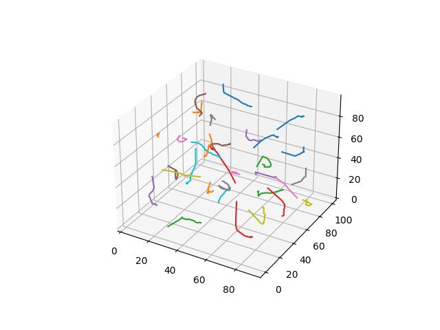
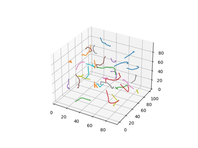
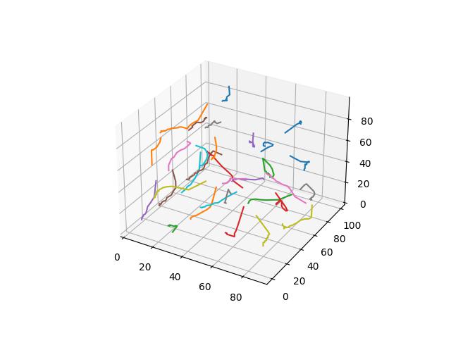
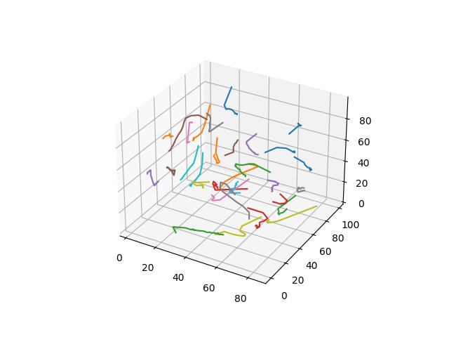
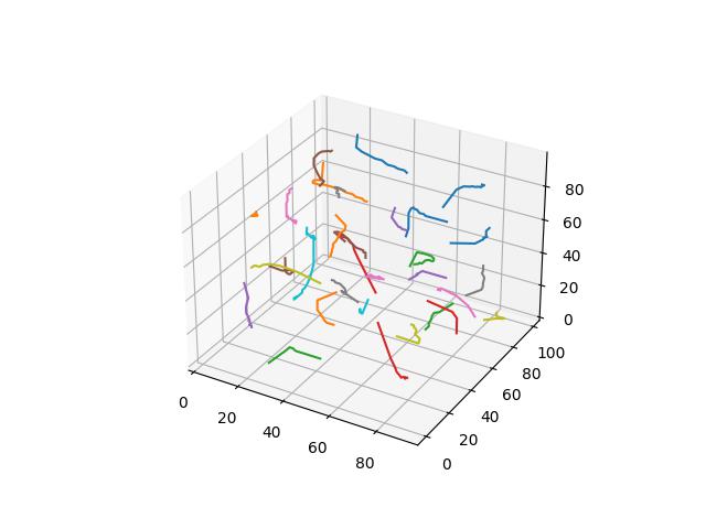
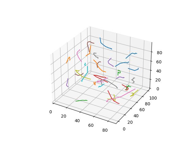
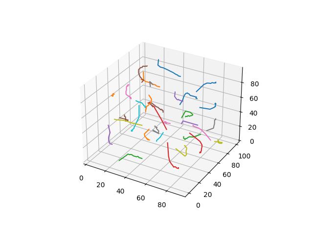
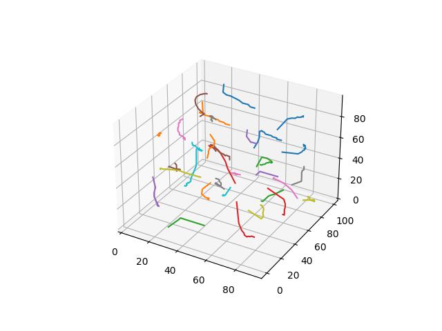
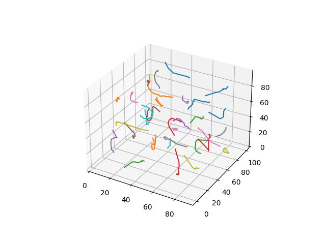
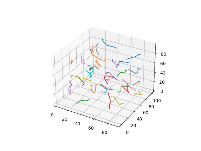
To demonstrate each distance function, we demonstate Voronoi relaxation in 2D and 3D space - as well as how those centers change position over time. For the Minowski and Yang metrics - for $p$ values of 3, 4, and 5 are demonstrated. Each cell is assigned a distinct color.
For 2D ($R^2$ space), GIFs show Voronoi relaxation for 100 iterations occuring on a 300x300 plane under each distance metric, starting from 32 randomly selected centers.
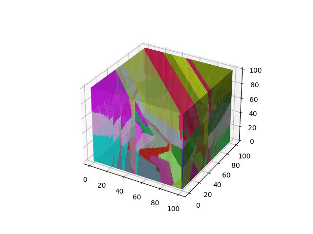
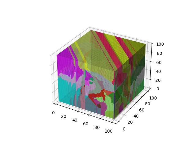
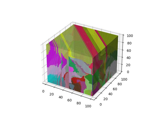
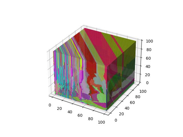
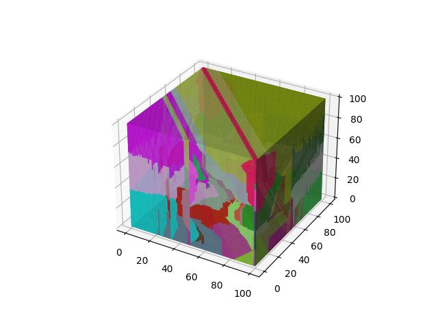
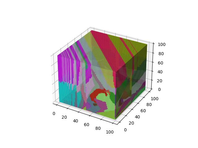
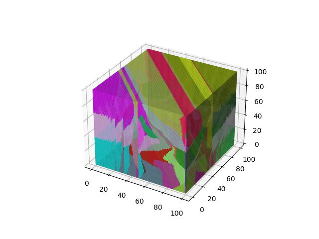
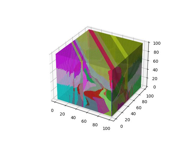
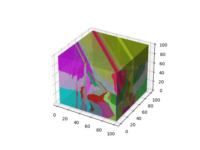
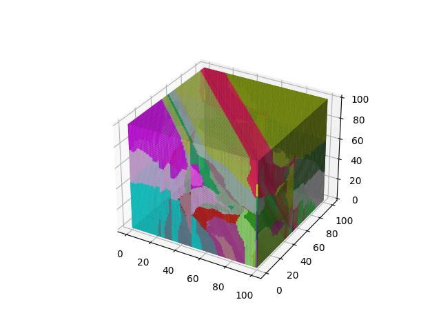
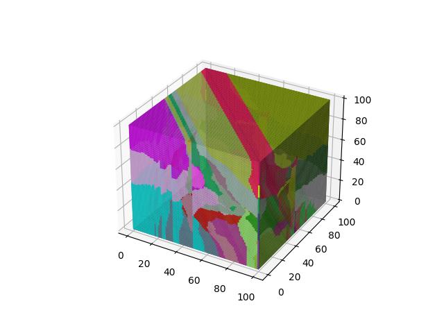
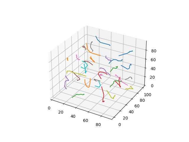
For 3D ($R^3$), images show the resulting Vornoi diagram after 100 iterations of Voronoi relaxation on a 100x100x100 space under each distance metric, starting from 32 randomly selected centers.
Euclidean
The most common distance function used with Voronoi diagrams (and in general), gives the length of the line between $x$ and $y$.
$$D(x,y)=\sqrt{\sum\limits_{i=1}^k (x_i-y_i)^2}$$

Manhattan
Probably the second most common distance function “in general”, giving the sum of the absolute differences between the corresponding elements of $x$ and $y$.
$$D(x,y)=\sum\limits_{i=1}^k \lvert x_i-y_i \rvert$$

Bray-Curtis / Sorenborg
While technically not a distance function due to not obeying the triangle inequality, it comes from biostatistics and related fields aiming to measure the how different two “sites” (says sites of animals). are on a per-element basis. Guaranteed to be between $[0,1]$ if all elements are positive.
$$D(x,y)=\frac{\sum\limits_{i=1}^k \lvert x_i-y_i \rvert}{\sum\limits_{i=1}^k \lvert x_i+y_i \rvert}$$

Canberra
A weighted version of Manhanttan distance, where the $i$-th element is weighted by the sum of the absolute value of $x_i$ and absolute value of $y_i$.
$$D(x,y)=\sum\limits_{i=1}^k \frac{\lvert x_i - y_i \rvert}{\lvert x_i \rvert + \lvert y_i \rvert}$$


Chebyshev
Also known as the maximum metric, defines distance as the maximum distance between any two of their corresponding elements of $x$ and $y$ ($x_1$ and $y_1$, $x_2$ and $y_2$, etc.).
$$D(x,y)=\max\limits_i (\lvert x_i - y_i \rvert)$$


Hellinger
Basically the Euclidean norm between the difference of the square root vectors of $x$ and $y$, more formally a version of a probability distribution similarity measure assuming $x$ and $y$ are discrete distributions.
$$D(x,y)=\frac{1}{\sqrt{2}}\sqrt{\sum\limits_{i=1}^k (\sqrt{x_i} - \sqrt{y_i})^2}$$


Minkowski
A generalization of the Manhattan and Euclidian distances by integer $p > 0$ ($p=1$ is Manhattan distance, $p=2$ is Euclidean). Measures distances on normed vector spaces.
$$D(x,y)=(\sum\limits_{i=1}^k \lvert x_i - y_i\rvert^p)^\frac{1}{p}$$
When $p=3$

When $p=4$

When $p=5$


Yang
A “newer” distance metric introduced for the purposes of retaining all the properties of distance metrics while being more useful than similarity measures used in high dimensional data (like cosine “distance”).
$$D(x,y)=((\sum\limits_{i:x_i\geq y_i} x_i - y_i)^p + (\sum\limits_{i:x_i < y_i} y_i - x_i)^p)^\frac{1}{p}$$
When $p=3$


When $p=4$

When $p=5$


Alternative Formulations
There exist many modifications to the original definitions of Voronoi diagrams and relaxation that can also lead to some interesting visual phenonena.
Perhaps one of the simplest modifications are k-th order Voronoi diagrams. Here instead of assigning points to cells based on their closest center, they are assigned to cells based on their 2-nd closest center, 3-rd closest, and so on ending at the $t$-th closest center (i.e. the furthest center). Formally we may also say, assigning based on the closest center (the original definition) is a 1-st order Vorinoi diagram.
Below we show resulting image for each distance measure as before, under the same 2D formulation. We opt for images instead of gifs here because for $k>1$, cells tend to split apart into smaller groups resulting in less visually cohesive iterations.
1-st Order
Euclidean
Manhattan
Bray-Curtis

Canberra

Chebyshev
Hellinger
Minkowski
$p=3$
$p=4$
$p=5$
Yang
$p=3$
$p=4$
$p=5$
-1-st Order
The $-1$-order occurs when points are added to cells based on the furthest center point. Generally the results under any distance formula are largely the same, only 2-4 cells emerge as most points have the same “furthest center point”.
Due to the aforementioned similarity across distace metrics, only the Euclidean and Manhattan distances are shown.